Image Segmentation

Deep Learning and Computer Vision in R: A Practical Introduction

SSA ACT workshop - Image Segmentation

Weihao (Patrick) Li

RSFAS, ANU

Content summary

• Overview of computer vision (CV)
• reticulate and torch basics
• Image classification, neural networks and Keras
• Convolutional neural networks
• Vision transformers
• Object detection
• > Image segmentation

Image segmentation

Image segmentation

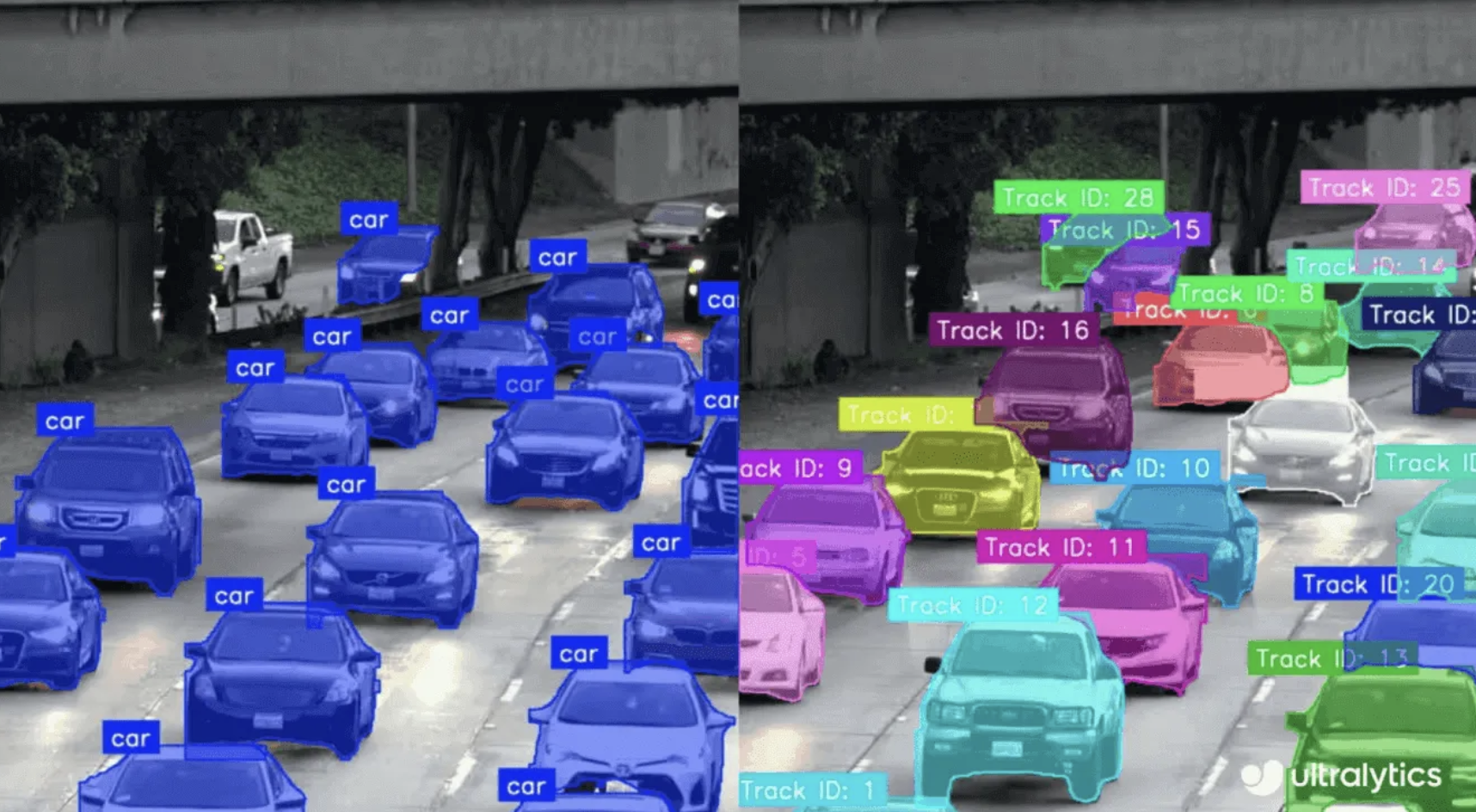
Image segmentation is the process of dividing an image into coherent regions so that pixels belonging to the same object or area are grouped together.

Where do we need segmentation?

• Medical imaging
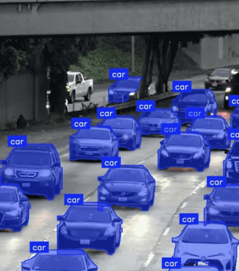
• Autonomous driving
• Agriculture/Phenotyping
• Robotics
• Video analysis
• Content editing
• …

Types of segmentation

• Semantic segmentation: Label each pixel with a class (no instance separation).

• Instance segmentation: Distinguish individual objects of the same class.

• Panoptic segmentation: Combines semantic + instance into one unified output.

Mask format

• Shape: (H, W) or (H, W, 1) a single channel per pixel
• Binary Segmentation: Pixel values: 0 (background), 1 (foreground)
• Multiclass Segmentation: Pixel values: 1, 2, … (class id)

Masks are commonly saved as greyscale PNG or TIFF on disk.

• Masks are integer labels, not normalized
• RGB masks should be converted to single-channel class IDs before training

YOLO format (instance segmentation)

• One text file per image.
• One row per object:
  • Object class index: An integer representing the class of the object (e.g., 0 for person, 1 for car, etc.).
  • Object bounding coordinates: The bounding coordinates around the mask area, normalized to be between 0 and 1.

<image_id>.txt:

<class-index> <x1> <y1> <x2> <y2> ... <xn> <yn>

COCO format (instance segmentation)

annotation.json:

• images: list of images
  • id: unique image ID
  • file_name: image filename
  • height, width: image size
• annotations: list of objects
  • image_id: links annotation to image
  • category_id: class of object
  • bbox: [x, y, width, height] (for object detection)
  • segmentation: polygon coordinates [[x1,y1, x2,y2, ...]] or run-length encoding for dense masks (object mask)
• categories: list of classes
  • id: class ID
  • name: class name

COCO/Mask to YOLO

The default COCO dataset includes segmentation annotations. If your custom dataset in COCO format also contains segmentation information, you can convert it to YOLO format for segmentation tasks.

ultralytics <- import("ultralytics", convert = FALSE)
convert_coco <- ultralytics$data$converter$convert_coco
convert_coco(labels_dir = "path/to/coco/annotations/",
             use_segments = TRUE)

Similarly, mask data can be converted into YOLO format.

convert_segment_masks <- ultralytics$data$converter$convert_segment_masks_to_yolo_seg
convert_segment_masks(masks_dir = "path/to/masks_dir", 
                      output_dir = "path/to/output_dir", 
                      classes = 80L)

Annotation tools

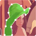
LabelMe: Web-based tool for creating polygonal and freehand annotations. Supports exporting to multiple formats like JSON for machine learning pipelines.

CVAT (Computer Vision Annotation Tool): Powerful open-source platform for image and video annotation. Supports polygons, masks, and tracking for object detection and segmentation.

VIA (VGG Image Annotator): Lightweight, browser-based tool. Ideal for quick annotations with minimal setup. Exports annotations in JSON or CSV.

Fully convolutional networks (2015)

Fully convolutional networks (FCNs) — Long, Shelhamer and Darrell (2015) — were the first deep learning architecture designed for semantic segmentation. They replace a classifier’s dense layers with convolutions, turning the final feature map into a spatial prediction of the image.

• Dense layers become convolutions, allowing arbitrary input sizes and producing a spatial map rather than a single label.
• The map is upsampled to the original image resolution, assigning a class label to every pixel.
• The predictions are often coarse because pooling and strided convolutions discard spatial detail that upsampling cannot recover. U-Net addresses this with skip connections that bring back fine-grained features.

U-Net family (2015 - present)

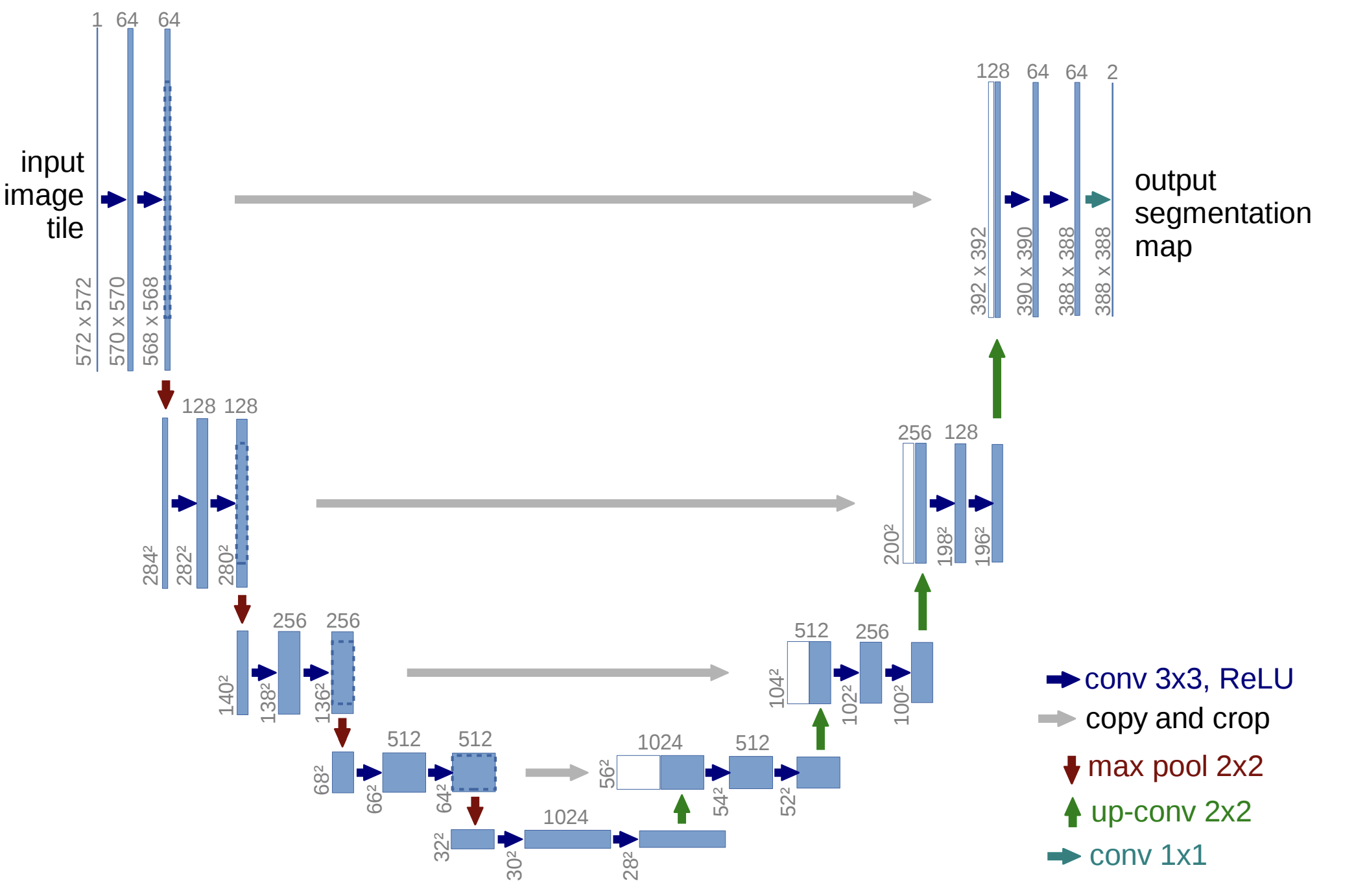
The U-Net family consists of encoder–decoder architectures with skip connections that preserve spatial detail, making them highly effective for dense prediction tasks in medical imaging, remote sensing, and agriculture.

Conv2DTranspose layer

YOLOv8 segmentation

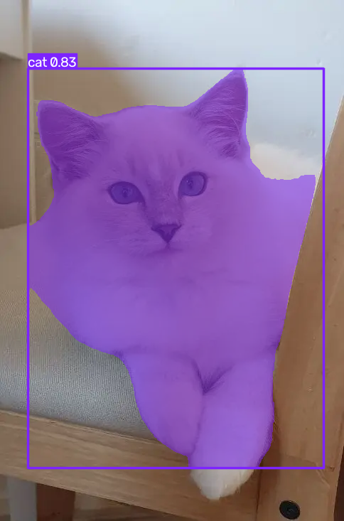
model <- ultralytics$YOLO("yolov8n-seg.pt") 
result <- model$predict("slide_figures/original.png")

image 1/1 /Users/patrickli/Desktop/rproj/ssa-cv-workshop/instructor/slides/slide_figures/original.png: 640x448 1 cat, 45.8ms
Speed: 3.7ms preprocess, 45.8ms inference, 7.4ms postprocess per image at shape (1, 3, 640, 448)

result[0]$save("slide_figures/cat_segmentation.png")

'slide_figures/cat_segmentation.png'

YOLOv8 segmentation training

Training a segmentation model in YOLO is very straightforward, and the data format is largely the same as for object detection.

model <- ultralytics$YOLO("yolov8n-seg.pt") 
results <- model$train(data = "carparts-seg.yaml", 
                       epochs = 100L, 
                       imgsz = 640L)
results <- model$predict("path/to/your/image.jpg")

Beyond the basics

The workshop covered classification, detection and segmentation. Four directions extend these foundations without requiring entirely new fundamentals:

• Foundation models — move beyond training a separate model for each class. SAM 2 segments objects based on prompts, while YOLO-World detects objects using open-vocabulary text prompts. Both are available through ultralytics, which is already loaded.
• Multimodal models — one of the fastest-moving areas in computer vision. CLIP matches images with free-form text, while VLMs (Qwen2-VL, LLaVA, GPT-4o) answer questions about images. Text prompts can also guide detection and segmentation, as in Grounded SAM.
• Generative models — diffusion models (Stable Diffusion, FLUX) and GANs generate synthetic images. In research, they can augment small datasets, serving a similar purpose to the Random* augmentation layers, but with learned image generation.
• Video and 3D — extend beyond individual images to temporal and spatial data. Tracking (ByteTrack) follows objects across frames, while action recognition identifies activities in video. Other directions include depth estimation, LiDAR and 3D medical imaging.

Thanks!

• TengMCing
• [email protected]
• https://patrickli.org